Example

In this chapter the Ball Thrower example GUI shipped with Simian GUI is described. For new users of Simian GUI the code of this example and the descriptions in this chapter may offer a good starting point to start using Simian GUI.

Ball Thrower

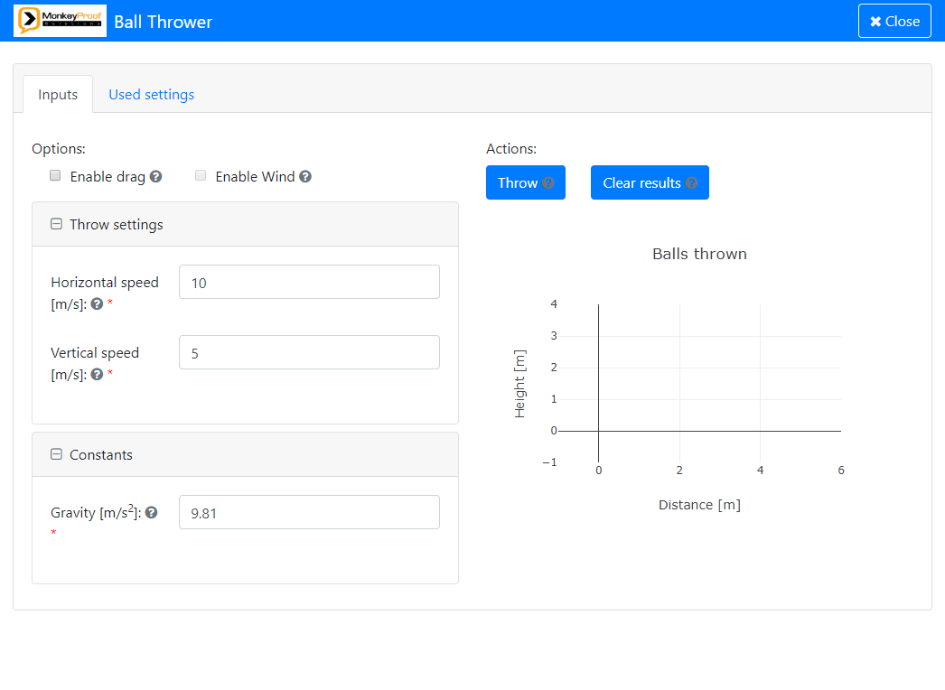
The Ball Thrower example contains a form that facilitates running a Ball Thrower simulation model. The model uses the MATLAB ode45 or scipy.integrate.solve_ivp solver to calculate the trajectory of the ball. The application upon startup looks as follows:

Ball Thrower Form

The model allows for simulating the throw of a ball in an idealised situation without drag and wind and can optionally be run to also simulate the effects of drag and wind on the ball.

The model also has inputs for the throw speed, ball radius, mass and drag coefficient, wind speed, gravity and air density. These inputs can be set from the form.

The following sections describe how to run this example, the most interesting features of the form and the physics and math behind the ball thrower model.

Running the example

To start the form in a pywebview window, make sure Simian GUI is on the Python path and run the following command in Python (ensure that pywebview is installed though, or you will get an error):

import simian.local
simian.local.Uiformio("simian.examples.ballthrower")

To run the Ball Thrower example in a local MATLAB session, ensure that Simian GUI and the Ball Thrower example files are on the MATLAB path and run the following command:

simian.local_v3_0_1.Uiformio("simian.examples_v3_0_1.ballthrower");

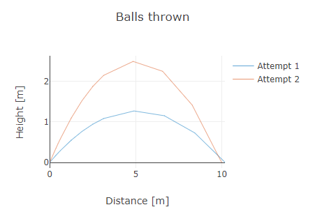
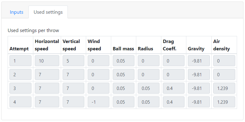
To simulate the throw of a ball, click the "Throw" Button. The trajectory of the ball will be shown in the plot and the settings are stored in the table in the "Used settings" tab. The speed with which the ball is thrown and the gravity can be modified to simulate the effect of these parameters on the trajectory of the ball. To simulate the effects of wind and/or drag on the throw, tick the corresponding options. These options will enable more settings that can be modified, which will have their own effect on the trajectory of the ball.

BallThrower files

The files making up the Ball Thrower example are stored in the simian-examples folder.

The form functions are in the ballthrower module:

ballthrower.py:
- gui_init: contains the form definition.
- gui_event: contains the callbacks of the throw and clear buttons and connects with the model to simulate the ball's trajectory.
logo.png: image shown in the header of the form.

The model for simulating a ball throw is in the ballthrower_engine module:

BallThrower: ballThrower class definition. Needs to be instantiated before you can call the throwBall method.
- _drag_ball: method creating the set of differential equations that need to be solved for the throw.
- throw_ball: method starting the simulation of the trajectory of the ball.
- _zero_crossing: method for determining the ground contact point boundary condition of the throw.

The MATLAB Ball Thrower contains the same functionality, but the functions have their own function files.

Features

The most interesting features of the example are discussed in the following subsections. Where possible code snippets from the example are included (sometimes slightly modified for readability) to illustrate how these features end up in code. The descriptions also contain links to other parts of the documentation where more information can be found.

We will discuss how the Ball Thrower example can conditionally enable and hide controls, conditionally override a value, add client side validation, prevent runs with invalid settings, and make parameters required. We will also show how to plot and tabulate data, add an image to the form and how we created the form's layout.

Conditionally enabled state

Wind cannot be simulated without simulating drag, as without drag the wind has no effect on the ball. To capture this in the form the "Enable wind" Checkbox is only enabled when the "Enable drag" checkbox is enabled.

Wind disabled when drag unticked.

To get this behaviour we set the disabled state of the "Enable wind" checkbox to true and add a Logic object to the "Enable wind" checkbox. Each Logic object needs a trigger and one or more actions. The trigger describes under which circumstances the actions in the logic object should be executed.

To ease disabling components with a trigger, the disableWhen method is available for each component. It uses the createDisableLogic function from the componentProperties package/module to disable the component when the trigger is triggered.

enable_wind_checkbox.disable_when(
    trigger_type="simple", trigger_value=["enableDrag", False]
)

enableWindCheckbox.disableWhen("simple", {"enableDrag", false})

Alternatively, when adding components from a table we can create a Logic object and put it in a dict/struct for the options column.

wind_logic = component_properties.create_disable_logic(
    trigger_type="simple", trigger_value=["enableDrag", False]
)
wind_options["logic"] = wind_logic

windLogic = componentProperties.createDisableLogic(...
    "simple", {"enableDrag", false});
windOptions.logic = windLogic;

Conditionally override a value

Disabling the "Enable wind" checkbox alone is not enough. It may already have been ticked, so we also need to ensure it is unticked when the "Enable drag" option is unticked.

For this we create an untick action. This action should change the checkbox's value property to false. We simply add this new action to the actions property of the existing Logic object of the "Enable wind" control, as it already has the correct trigger for this action.

wind_logic.actions.append(
    {
        "type": "value",
        "value": "value = false"
    }
)

windLogic.actions{end + 1} = struct( ...
    "type", "value",  ...
    "value", "value = false");

Conditionally hide controls

When drag and or wind are disabled, the controls for the ball properties and the wind speed are not needed and can be hidden. For this we do not use a Logic object, but a Conditional object which has a more concise definition. First the Conditional object is created with the control we want to hide as input. Then we put the key of the control the hiding depends on in the when property. The value of that control for which our control is to be hidden is put in the eq property.

The following statements hide the ballPanel Panel when the "Enable drag" checkbox is unticked:

# Hide ball panel when drag is not enabled.
drag_enabled = component_properties.Conditional(ballPanel)
drag_enabled.when = "enableDrag"
drag_enabled.eq = False

# Or when using table's 'options' column:
ball_options = {"conditional": {"when": "enableDrag", "eq": False}}

% Hide ball panel when drag is not enabled.
ballCondition       = componentProperties.Conditional(ballPanel);
ballCondition.when  = "enableDrag";
ballCondition.eq    = false;

% Or when using table's 'options' column:
ballOptions.conditional.when = "enableDrag";
ballOptions.conditional.eq   = false;

When controls are hidden, their values are not included in the payload that is sent to the back-end. To ensure that values of hidden controls are included in the payload and user defined values persist when the control is (temporarily) hidden, set the clearOnHide property of the control to false (default is true).

ball_radius.clearOnHide = False

ballRadius.clearOnHide = false;

Client side validation

For some controls we need to limit the range of values that can be entered. The ball's radius for instance should not be negative. To enforce this we can add a Validate object to a control. For the ball radius text field we create a Validate object with the control as input and set the min property to zero. This will ensure that when negative values are entered an error message is shown to highlight the problem.

This type of validation can also be done in the back-end, but doing it in the form provides quicker feedback and shows it close to the invalid value:

Invalid ball radius detected.

# Allow values greater than 0.
ball_radius_validate = component_properties.Validate(ballRadius)
ball_radius_validate.min = 0

# Or when using table's 'options' column:
radius_options = {"validate": {"min":  0}}

% Allow values greater than 0.
radiusValidate      = componentProperties.Validate(ballRadius);
radiusValidate.min  = 0;

% Or when using table's 'options' column:
radiusOptions.validate.min = 0;

Prevent run with invalid settings

To prevent running the model with values that are flagged invalid by the validation the "Throw" Button is disabled. This can simply be done by setting the disableOnInvalid property of the throw button control to true. This ensures that when the validations in the form detects an invalid value, the throw button is automatically disabled and only enabled again when all values in the form are valid.

Throw button disabled.

throw_button.disableOnInvalid = True

throwButton.disableOnInvalid = true;

Required parameters

When empty values are not allowed for a setting, using the setRequired() method of the component will ensure that empty values are marked invalid. The setRequired() method creates a Validate object for the control (if none exist yet) and sets the required property to true (default is false). When you add a new Validate object to the control after using the setRequired() method, the control will lose its required state. Alternatively you can directly set the required property of the Validate object to true.

Controls that have a required value are indicated with a red asterisk and empty values are marked invalid.

Throw button disabled.

ball_radius = component.Number("ballRadius")
ball_radius.setRequired()

# or
ball_radius_validate = component_properties.Validate(ball_radius)
ball_radius_validate.required = True

# Or when using table's 'options' column:
radius_options["validate"].update({"required": True})

ballRadius = component.Number("ballRadius");
ballRadius.setRequired();

% or 

ballRadiusValidate = componentProperties.Validate(ballRadius);
ballRadiusValidate.required = true;

% Or when using table's 'options' column:
radiusOptions.validate.required = true;

Plotting results

To plot ball trajectories in the form after clicking the "Throw" button, we add a Plotly object in the definition of the form and set its "title", "xaxis" and "yaxis" properties to make it look nicer:

Initialized plot axes.

# Create a plot window to plot the ball trajectories in.
my_plot = component.Plotly("plot", column_2)
my_plot.defaultValue['data'] = []
my_plot.defaultValue['layout'] = {
    "title": {"text": "Balls thrown"}, 
    "xaxis": {"title": "Distance [m]"},
    "yaxis": {"title": "Height [m]"},
    "margin": {"t": 40, "b": 30, "l": 50}
}
my_plot.defaultValue['config'] = {
    "displaylogo": False
}

% Create a plot window to plot the ball trajectories in.
myPlot                      = component.Plotly("plot", column_2);
myPlot.defaultValue.data    = {};
myPlot.defaultValue.layout  = struct(...
    "title", struct("text", "Balls thrown"), ...
    "xaxis", struct("title", "Distance [m]"), ...
    "yaxis", struct("title", "Height [m]")); 
myPlot.defaultValue.config  = struct(...
    "displaylogo", false);

To plot a ball trajectory in the form we create a Plotly object from the data in the form via the getSubmissionData utility function. We can then use the Plotly Figure.add_scatter() method (Python) or utils.Plotly.plot() method (MATLAB) to plot the x and y values that were returned by the BallThrower model. We then put the Plotly object in the payload using the setSubmissionData utility function. In MATLAB we can extend the legend by first getting its existing values and then recreating the legend with the existing and new values. In Python the legend is automatically extended with the name of the added scatter trace.

Visualisation of ball trajectories.

# Create a Plotly object from the information in the payload.
plot_obj = utils.getSubmissionData(payload, key='plot')[0]

# Plot the new newly calculated x and y values, append the legend and put the plotly
# object in the submission data.
nr = len(plot_obj.figure.data) + 1
plot_obj.figure.add_scatter(x=x, y=y, name=f"Attempt {nr}", mode="lines")
utils.setSubmissionData(payload, key='plot', data=plot_obj)

% Create a plotly object from the data in the form, put the current data in the plotly
% object and get the legends.
plotly          = utils.getSubmissionData(payload, "plot");
dataSpec        = plotly.data;
existingNames   = cellfun(@(x) x.name, plotly.data, "UniformOutput", false);

% Plot the newly calculated x and y values, append the legend and put the plotly
% object in the submission data.
nr = numel(dataSpec) + 1;
plotly.plot(x, y)
plotly.legend(existingNames{:}, sprintf("Attempt %d", nr));
payload = utils.setSubmissionData(payload, "plot", plotly);

Tabulating used settings

To keep track of the settings used for the simulations of the throws, we can add them to a table. In the form definition we create a DataGrid and use its setContent method to add nine non-editable columns with TextFields.

# Create a table to store the throw settings in.
table_out = component.DataGrid("summary", tab_b)
table_out.setContent(
    labels=["Attempt", "Horizontal speed", "Vertical speed", "Wind speed", "Ball mass",
            "Radius","Drag Coeff.", "Gravity", "Air density"],
    keys=["nr", "u0", "v0", "w", "m", "r", "Cd", "g", "rho"],
    component_types=["TextField"] * 9,
    is_editable=[False] * 9)
table_out.label = "Used settings per throw"

% Create a table to store the throw settings in.
tableOut        = component.DataGrid("summary", tabB);
tableOut.label  = "Used settings per throw";
tableOut.setContent(...
    ["Attempt", "Horizontal speed", "Vertical speed", "Wind speed", "Ball mass", ...
    "Radius", "Drag Coeff.", "Gravity", "Air density"], ...
    ["nr", "u0", "v0", "w", "m", "r", "Cd", "g", "rho"], ...
    repmat("TextField", 1, 9), ...
    false(1, 9));

When the Throw button is clicked we create a new row with the settings that were used in the simulation. This new row is appended to the values already in the table and using the setSubmissionData() function in the utils, it is added to the payload that will be sent to the form.

DataGrid filled with data.

# Update the table with the settings used for the throws.
new_row = [nr, hor_speed, ver_speed, wind_speed, mass_ball, radius_ball, drag_coeff,
            gravity, rho_air]

if nr == 1:
    # First throw. Only put the new row in the table.
    new_table_values = [new_row]
else:
    # Extra row. Append the row to the DataFrame from the submission data.
    new_table_values = utils.getSubmissionData(payload, key="summary")[0]
    new_table_values = new_table_values.append(
        DataFrame(data=[new_row], columns=new_table_values.columns))

utils.setSubmissionData(payload, key="summary", data=new_table_values)

% Update the table with the settings used for the throws.
newRow = {nr, horSpeed, verSpeed, windSpeed, massBall, radiusBall, dragCoeff, ...
    gravity, rhoAir};

if nr == 1
    % First throw. Only put the new row in the table.
    newTableValues  = newRow;
else
    tableValues     = sub_getTableValues(payload, "summary");
    newTableValues  = [tableValues; newRow];
end

payload = utils.setSubmissionData(payload, "summary", newTableValues);

Layout of controls

Controls in the form can be laid out using panels, containers, columns, tables and tabs.
Panels allow for grouping controls and allow for hiding them by collapsing the panel.
Containers allow for grouping controls without adding borders or background colors.
Columns allow for putting controls and panels next to each-other, making better use of the space in the form. When the window containing the form gets smaller, the contents of the columns are placed below each-other to reduce horizontal scrolling. Tables allow for laying components out in a grid. Tabs allow for grouping and showing/hiding larger parts of the form.

Background

In this section the physics and math side of throwing a ball are discussed for an idealized situation without drag and wind, and for situations where drag, and wind and drag are simulated.

Idealized situation

Let"s throw a ball in an ideal world without drag and wind. Defining a starting point, throwing speed and gravitation will do the trick:

\[\sum \vec{F} = m \cdot \vec{g},\]

therefore, we can derive that:

\[ \begin{align} x & = u_0 t \\ y & = v_0 t - \frac{1}{2}gt^2 \end{align} \]

This can be solved analytically:
\[ \frac{d^2}{dt^2} \begin{bmatrix} x \\ y \end{bmatrix} = \begin{bmatrix} 0 \\ -g \end{bmatrix} \]

The begin position and speed are enough to determine the final result:
\[x_0, y_0, u_0, v_0\]

Such that:
\[ \begin{align} x(t) & = x_0 + u_0 t \\ y(t) & = y_0 + v_0 t - \frac{1}{2}gt^2 \\ u(t) & = u_0 \\ v(t) & = v_0 - gt \\ \end{align} \]

Adding drag

When we add drag to the idealized situation, things become more complicated:

\[\vec{F}_{drag} = -\frac{1}{2} \rho A |\vec{v}|^2 C_d \hat{v} \]

And thus: \[\sum \vec{F} = \vec{F}_{drag} + \vec{F}_g.\]

This can no longer be solved analytically, this can only be solved numerically. Therefore we need to solve the following equations using a differential equation solver.

\[ \dfrac{d}{dt} \begin{bmatrix} x \\ \dot{x} \\ y \\ \dot{y} \end{bmatrix} = \begin{bmatrix} \dot{x} \\
-\frac{1}{2m} \rho \dot{x}^2 C_d A \dfrac{\dot{x}}{|\dot{x}|} \\
\dot{y} \\
-\frac{1}{2m} \rho \dot{y}^2 C_d A \dfrac{\dot{y}}{|\dot{y}|} + g \end{bmatrix} \]

The begin position and speed are not enough to determine the final result:
\[x_0, y_0, u_0, v_0\]

For this situation we need more parameters:

\( m \): Mass of the ball
\( \rho \): Air density
\( r \): Area of the surface, assumed a sphere here, so radius is asked

Adding wind

When we add wind, the equations become slightly more complicated.

\[\vec{F}_{drag + wind} = -\frac{1}{2} \rho A |\vec{v_r}|^2 C_d \hat{v_r} \]

where \(\vec{v_r} = \vec{v} + \vec{w}\), and

\[\sum \vec{F} = \vec{F}_{drag + wind} + \vec{F}_g.\]

The equations using that need to be solved with the ode45 solver become:

\[ \dfrac{d}{dt}\begin{bmatrix} x \\ \dot{x} \\ y \\ \dot{y} \end{bmatrix} = \begin{bmatrix} \dot{x} \\
-\frac{1}{2m} \rho (\dot{x} - w)^2 C_d A \dfrac{\dot{x} - w}{|\dot{x} - w|} \\
\dot{y} \\
-\frac{1}{2m} \rho \dot{y}^2 C_d A \dfrac{\dot{y}}{|\dot{y}|} + g \end{bmatrix} \]

The begin position and speed are not enough to determine the final result: \[x_0, y_0, u_0, v_0\]

For this situation we need more parameters:

\( m \): Mass of the ball
\( \rho \): Air density
\( r \): Area of the surface, assumed a sphere here, so radius is asked
\( w \): Wind Speed

Simian GUI Documentation v3.1.0